
Black Monday: How unlikely was it, and could it happen again? (Part I)
This post is the first in a series that will look back on the events of Black Monday, which happened 30 years ago today, and explore how it might be relevant to contemporary investing. It makes for a fascinating educational case study that weaves together lessons in finance, statistics, coding, and history. Throughout this series, I'll be “showing my work” with R code that you can run yourself. (For example, in RStudio)
The S&P 500 had seen a new all-time high only six weeks previously, but the week of October 12th, 1987 did not go well for the US stock market. After Monday and Tuesday saw a small loss followed by a small gain, the rest of the week saw mounting losses: 3% on Wednesday, 2% on Thursday, and an alarming and very unusual 5% on Friday.
Still, few were prepared for what happened when the market re-opened on Monday the 19th. The S&P 500 began falling quickly after the open, and continued to do so almost unabated throughout the entire trading day. (See this WSJ interactive for how things unfolded during the day.) When the dust settled at the close, the index had dropped an astonishing 20%. This drop was and continues to be unprecedented; at no other time in its 60-year history has the index dropped even half as much. Monday the 19th, 1987 has since become known as “Black Monday”, one of only a handful of trading dates to receive names and by far the most well known.
As with all disasters, a natural question to ask is, “could it happen again?” As it turns out, there are a number of different ways to try to answer this question, some of which do a good job of highlighting the challenges and complexities of mathematical finance.
To address the question, “how likely would a repeat (or worse) of Black Monday be?”, you need two things:
(1) A model for the probability that the market will rise or fall by a given amount,
(2) Data for the model, and
(3) Knowledge of the ways in which your model may be imprecise or incomplete.
So, let's begin.
The most basic model commonly used for the distribution of price changes is the log-normal distribution. This model assumes that the change of the natural logarithm of price ( log pt1 - log pt0 ) is normally distributed.
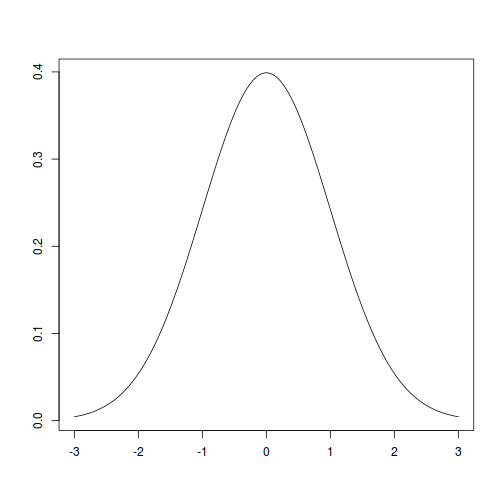
The formula for the normal distribution is
 = \frac{1}{\sqrt{\tau\sigma^2} } \; e^{ -\frac{(x-\mu)^2}{2\sigma^2} }")
…where τ=2π is the circle constant and μ and σ are the distribution's two parameters, which govern where the peak of the distribution is centered, and how wide it is. For the most basic case of μ=0 and σ=1, the curve looks like this:
x.range <- seq(-3,3,0.01)
plot(x=x.range,y=dnorm(x.range),type="l",xlab="",ylab="")
Now we need to see what real-world data looks like. Conveniently, Yahoo! has a freely-available daily timeseries for the S&P 500.1
Let's load the data series. Specifically, we'll make one set of data that starts on the official index inception date of March 4, 19572, and ends the day before Black Monday. Then we'll make one more datapoint for Black Monday's return. What does the data look like?
library(quantmod)
library(xts)
library(PerformanceAnalytics)
sp500 <- getSymbols(Symbols="^GSPC",
                    auto.assign=FALSE,
                    from="1957-03-04",
                    to=  "1987-10-20")
sp500.hist <- sp500$GSPC.Close["1957-03-04/1987-10-16",]
chart.TimeSeries(sp500.hist,
                 main="S&P 500 daily history",
                 ylab="Index Value")
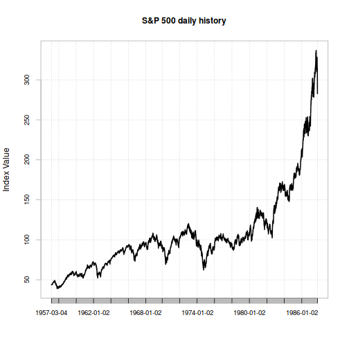
For this data, μ=0.000241 and σ=0.00797. For this model, we can determine how likely Black Monday was by plugging in μ, σ, and the desired cutoff value (-0.22 or -22%) into the cumulative distribution function, which will then return the total probability of observing a return that extreme or worse.
sp500.hist.ret.xts <- diff(log(sp500.hist))[is.finite(diff(log(sp500.hist)))]
sp500.hist.ret <- as.numeric(sp500.hist.ret.xts)
sp500.hist.mu <- mean(sp500.hist.ret)
sp500.hist.sd <- sd(sp500.hist.ret)
sp500.bm.ret <- as.numeric(diff(log(sp500$GSPC.Close))["1987-10-19",])
1/pnorm(q=sp500.bm.ret,mean=sp500.hist.mu,sd=sp500.hist.sd)
## [1] 4.03487e+181
So, we'd expect an event as extreme as Black Monday every 4.03 × 10181 trading days.
On the one hand, this explains why the event was such a surprise… the most-commonly-assumed model indicates it was very unlikely! If you're curious about where quotes like “this was an 17 (or 25, etc.) sigma event” come from, take σ and divide it into the % price change to get the number of standard deviations of the move - in this case roughly 29.
On the other hand… while Black Monday may have been unlikely, was it really that unlikely? According to current estimates the universe is only 3.46 × 10¹² trading days old. Was Black Monday really so unlikely that we'd only expect to see it once in 10169 lifetimes of the universe? Something seems fishy here. Given the frequency with which “Black Swan”, “Unprecedented” events seem to happen in finance, perhaps we can do better than say this was so unlikely as to never happen again, declare victory, and walk away.
To see how we might do better, click over to the next article.
1: Yahoo!'s data series for the S&P 500 doesn't include dividends, but since we're looking at extreme 1-day changes, we can safely ignore their impact in this case – the contribution to returns of dividends is quite small and stable at the daily time scale.
2: For dates before 1962-01-02, the Yahoo! series only has close values; other dates have all of Open, High, Low, and Close. We only use the close prices for these exercises.