Black Monday: How unlikely was it, and could it happen again? (Part III)
This post is the third in a series that will look back on the events of Black Monday, which happened 30 years ago today, and explore how it might be relevant to contemporary investing. Click here to read the first post and here to read the second.
We saw in the last post that while the Student-t distribution fits daily market returns better than the normal distribution, it cannot model the observation that market volatility tends to cluster, with some time periods having higher and others lower typical daily movements.
The most straightforward and commonly-used method for modeling time-varying volatility is the so-called GARCH (.pdf) method. In its basic form, it builds an estimate of volatility for a given point in time out of three pieces:
(1) a constant term, to which volatility tends to revert
(2) the previous period's realized volatility
(3) the previous period's volatility estimate
The overall formula looks like this:
The formula has three parameters: omega, alpha, and beta.
So, let's fit the model. We'll assume that any any given point in time, returns are normally distributed with a zero mean. The resulting model parameters are:
library(rugarch)
spec <- ugarchspec(variance.model=list(model="sGARCH"),
                   mean.model=list(armaOrder=c(0,0),include.mean=FALSE),
                   distribution.model="norm")
thisFit <- ugarchfit(spec=spec,data=as.numeric(sp500.hist.ret))
coef(thisFit)
##        omega       alpha1        beta1
## 5.136072e-07 8.088055e-02 9.143174e-01
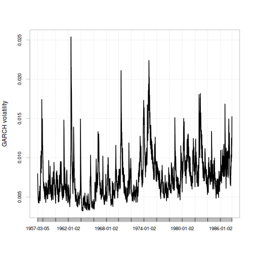
Fitting them to the data gives a time-varying volatility estimate leading up to Black Monday that looks like this:
spec <- ugarchspec(variance.model=list(model="sGARCH"),
                   mean.model=list(armaOrder=c(0,0),include.mean=FALSE),
                   distribution.model="norm",
                   fixed.pars = as.list(coef(thisFit)))
thisFilter <- ugarchfilter(spec=spec,data=sp500.hist.ret.xts)
chart.TimeSeries(xts(thisFilter@filter$sigma,index(sp500.hist.ret.xts)),ylab="GARCH volatility")

Since the volatility estimate for any period only depends on the previous period's values for returns and volatility, all we need to do to get the GARCH model's estimate for the volatility on Black Monday is use the values at the very end of the series.
n <- length(sp500.hist.ret)
bm.garch.pred.sigma <- as.numeric(sqrt(coef(thisFit)["omega"] +
                                       coef(thisFit)["alpha1"]*(sp500.hist.ret[n])^2 +
                                       coef(thisFit)["beta1"]*thisFilter@filter$sigma[n]^2))
1/pnorm(q=sp500.bm.ret,mean=0,sd=bm.garch.pred.sigma)
## [1] 2.097829e+27
Hrm. The basic GARCH model, compared to the Normal distribution model, says that Black Monday was much more likely. However, the result it gives still seems very unrealistic.
Well, can we combine the two approaches of a Student-t distribution and GARCH time-varying volatility? Yes:
spec <- ugarchspec(variance.model=list(model="sGARCH"),
                   mean.model=list(armaOrder=c(0,0),include.mean=FALSE),
                   distribution.model="std")
thisFit <- ugarchfit(spec=spec,data=sp500.hist.ret)
coef(thisFit)
##        omega       alpha1        beta1        shape
## 4.965783e-07 7.661085e-02 9.184568e-01 9.197535e+00
spec <- ugarchspec(variance.model=list(model="sGARCH"),
                   mean.model=list(armaOrder=c(0,0),include.mean=FALSE),
                   distribution.model="std",
                   fixed.pars = as.list(coef(thisFit)))
thisFilter <- ugarchfilter(spec=spec,data=sp500.hist.ret.xts)

bm.garch.pred.sigma <- as.numeric(sqrt(coef(thisFit)["omega"] +
                                       coef(thisFit)["alpha1"]*(sp500.hist.ret[n])^2 +
                                       coef(thisFit)["beta1"]*thisFilter@filter$sigma[n]^2))
1/pnst(q=sp500.bm.ret,l=0,s=bm.garch.pred.sigma,df=coef(thisFit)["shape"])
## [1] 1644627
…and the result is an implied probability of a Black Monday-scale event once every 1,644,627 trading days - that is, about once every 6,000 to 7,000 years.
Of the four approaches to modeling volatility that we've tried in this series of articles, this approach gives the highest probability… though that probability is still very low.
For conclusions, click over to the next article.
