Author: Ian Erickson

Black Monday: How unlikely was it, and could it happen again? (Part IV)

This post is the fourth in a series that will look back on the events of Black Monday, on the occasion of its 30th anniversary, and explore how they might be relevant to contemporary investing. Click here to read the first post, here to read the second, and here to read the third.

In this series of articles, we've looked at a number of quantitative methods for answering the question “at the time it occurred, how likely was a market crash on the scale of Black Monday?”

(Of course, it's possible to model volatility in arbitrarily complicated ways - we've just had a look at the lowest-hanging fruit in this overview series.¹)

The four answers from the approaches we used range from “basically impossible” for the normal distribution method, to “about once every six to seven thousand years” for the method that combines time-varying volatility with the Student-t distribution.

Since Black Monday did, in fact, happen - but hasn't happened since - I would lean towards asserting that the model which gives the highest probability is probably the one that will be the most accurate going forward.²

This naturally leads to the question of how likely another event like Black Monday would be today. As we mark the 30th anniversary, volatility has actually been unusually low by historical standards - so much so that there's a fair amount of concern about the market's lack of concern.

But all four of these methods are easy to use to make a prediction about today: just extend the input data to the present. If you do so, you'll see that both of the static methods indicate a higher probability of a Black Monday event now than they did when just looking at data from before the event. This is because since the event happened, both models show a higher probability of it. (In fact, the static Student-t method indicates such an event should happen roughly once every 300 years.) On the other hand, both of the dynamic (GARCH) methods indicate that the likelihood of another Black Monday event right now is very low - since while Black Monday did happen, it happened a long time ago and recent market volatility has been very subdued, unlike the increasing turmoil in the weeks leading up to Black Monday.

So, what are the takeaways from this exercise?

1. The probability estimate you get depends on the model you use.
2. Overall historical probability of an event can differ from the probability of that event at a particular point in time.
3. While Black Monday was very improbable by any measure, time-varying volatility models did indicate that market risk was growing.
4. The normal distribution is probably a bad choice to model extreme events. (Though it may be fine for answering other questions.)
5. While an event on the scale of Black Monday may occur every century or two, it's fairly unlikely at the moment since recent volatility has been low.

This concludes the series… I hope you've found it interesting and useful. Feel free to drop us a line if you have questions or comments.

Further reading:

The book “A First-Class Catastrophe: The Road to Black Monday, the Worst Day in Wall Street History” has recently been released. It's an in-depth account of the events of Black Monday, and While I haven't read it yet myself the reviews look good.

The market is constantly providing lessons to be learned. Here's a good one for quants, related to Black Monday.

Bloomberg has a great retrospective with commentary from many leading names in finance that you can check out here.

1: For example, you could fit an assymetric distribution to trailing returns, or use market-implied volatility from options prices instead of trailing returns.
2: I believe that all four approaches shown in this series are simple enough that given the amount of input data, overfitting is not likely to be a serious concern.

Black Monday: How unlikely was it, and could it happen again? (Part III)

This post is the third in a series that will look back on the events of Black Monday, which happened 30 years ago today, and explore how it might be relevant to contemporary investing. Click here to read the first post and here to read the second.

We saw in the last post that while the Student-t distribution fits daily market returns better than the normal distribution, it cannot model the observation that market volatility tends to cluster, with some time periods having higher and others lower typical daily movements.

The most straightforward and commonly-used method for modeling time-varying volatility is the so-called GARCH (.pdf) method. In its basic form, it builds an estimate of volatility for a given point in time out of three pieces:

(1) a constant term, to which volatility tends to revert
(2) the previous period's realized volatility
(3) the previous period's volatility estimate

The overall formula looks like this:

The formula has three parameters: omega, alpha, and beta.

So, let's fit the model. We'll assume that any any given point in time, returns are normally distributed with a zero mean. The resulting model parameters are:

library(rugarch)
spec <- ugarchspec(variance.model=list(model="sGARCH"),
                   mean.model=list(armaOrder=c(0,0),include.mean=FALSE),
                   distribution.model="norm")
thisFit <- ugarchfit(spec=spec,data=as.numeric(sp500.hist.ret))
coef(thisFit)

##        omega       alpha1        beta1 
## 5.136072e-07 8.088055e-02 9.143174e-01

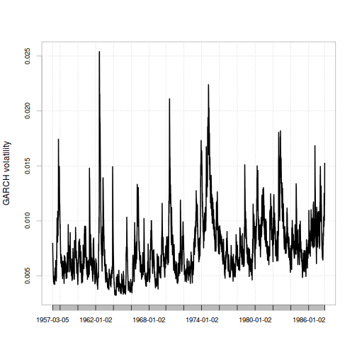
Fitting them to the data gives a time-varying volatility estimate leading up to Black Monday that looks like this:

spec <- ugarchspec(variance.model=list(model="sGARCH"),
                   mean.model=list(armaOrder=c(0,0),include.mean=FALSE),
                   distribution.model="norm",
                   fixed.pars = as.list(coef(thisFit)))
thisFilter <- ugarchfilter(spec=spec,data=sp500.hist.ret.xts)
chart.TimeSeries(xts(thisFilter@filter$sigma,index(sp500.hist.ret.xts)),ylab="GARCH volatility")

Since the volatility estimate for any period only depends on the previous period's values for returns and volatility, all we need to do to get the GARCH model's estimate for the volatility on Black Monday is use the values at the very end of the series.

n <- length(sp500.hist.ret)
bm.garch.pred.sigma <- as.numeric(sqrt(coef(thisFit)["omega"] +
                                       coef(thisFit)["alpha1"]*(sp500.hist.ret[n])^2 +
                                       coef(thisFit)["beta1"]*thisFilter@filter$sigma[n]^2))
1/pnorm(q=sp500.bm.ret,mean=0,sd=bm.garch.pred.sigma)

## [1] 2.097829e+27

Hrm. The basic GARCH model, compared to the Normal distribution model, says that Black Monday was much more likely. However, the result it gives still seems very unrealistic.

Well, can we combine the two approaches of a Student-t distribution and GARCH time-varying volatility? Yes:

spec <- ugarchspec(variance.model=list(model="sGARCH"),
                   mean.model=list(armaOrder=c(0,0),include.mean=FALSE),
                   distribution.model="std")
thisFit <- ugarchfit(spec=spec,data=sp500.hist.ret)
coef(thisFit)

##        omega       alpha1        beta1        shape 
## 4.965783e-07 7.661085e-02 9.184568e-01 9.197535e+00

spec <- ugarchspec(variance.model=list(model="sGARCH"),
                   mean.model=list(armaOrder=c(0,0),include.mean=FALSE),
                   distribution.model="std",
                   fixed.pars = as.list(coef(thisFit)))
thisFilter <- ugarchfilter(spec=spec,data=sp500.hist.ret.xts)

bm.garch.pred.sigma <- as.numeric(sqrt(coef(thisFit)["omega"] +
                                       coef(thisFit)["alpha1"]*(sp500.hist.ret[n])^2 +
                                       coef(thisFit)["beta1"]*thisFilter@filter$sigma[n]^2))
1/pnst(q=sp500.bm.ret,l=0,s=bm.garch.pred.sigma,df=coef(thisFit)["shape"])

## [1] 1644627

…and the result is an implied probability of a Black Monday-scale event once every 1,644,627 trading days - that is, about once every 6,000 to 7,000 years.

Of the four approaches to modeling volatility that we've tried in this series of articles, this approach gives the highest probability… though that probability is still very low.

For conclusions, click over to the next article.

Black Monday: How unlikely was it, and could it happen again? (Part II)

This post is the second in a series that will look back on the events of Black Monday, which happened 30 years ago today, and explore how it might be relevant to contemporary investing. Click here to read the first post.

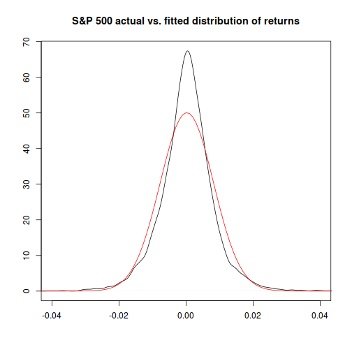
Looking at the normal distribution we've calculated, versus the actual distribution of returns, gives a clue as to what might have gone wrong with our first prediction of how unlikely Black Monday was:

plot(density(sp500.hist.ret),xlim=c(-0.04,0.04),xlab="",ylab="",
     main="S&P 500 actual vs. fitted distribution of returns")
x.range <- seq(-0.05,0.05,0.001)
points(x=x.range,
       y=dnorm(x.range, mean=sp500.hist.mu, sd=sp500.hist.sd),
       type="l", col="red")

Hmm. It looks like the normal distribution is an OK, but not a great, fit to the actual observed one.¹

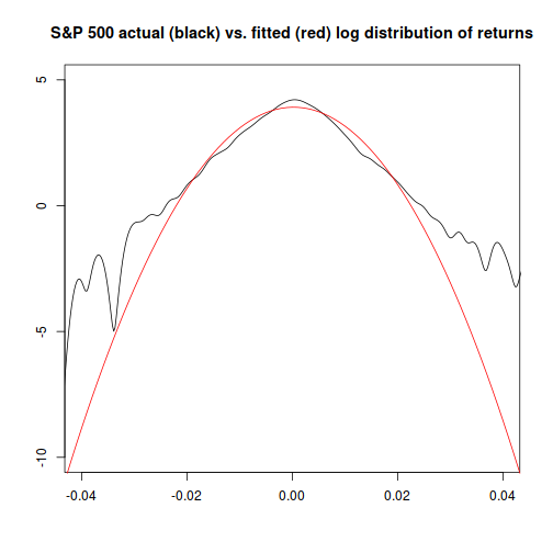
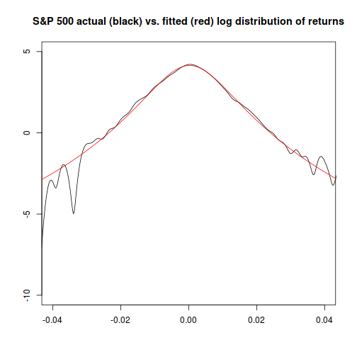
And, if we plot the log of probability for each distribution, we can see that the relative difference between them is largest at extreme values:

plot(x=density(sp500.hist.ret)$x,y=log(density(sp500.hist.ret)$y),
     xlim=c(-0.04,0.04),ylim=c(-10,5),xlab="",ylab="",
     main="S&P 500 actual (black) vs. fitted (red) log distribution of returns",type="l")
points(x=x.range,y=log(dnorm(x.range, mean=sp500.hist.mu, sd=sp500.hist.sd)), type="l", col="red")

Since we're trying to determine what the probability is at an extreme value, the fact that the normal distribution becomes an increasingly worse fit for more extreme values is a big problem. This is a reason why quants are often warned against blind use of the normal distribution: it can give you bad answers just when you can least afford them.²

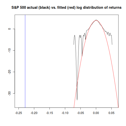
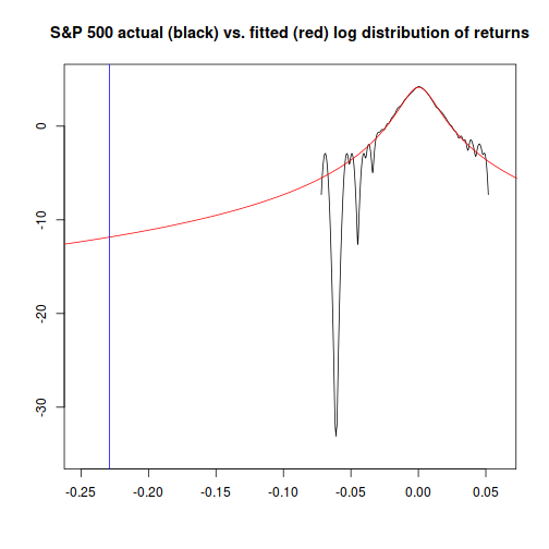
The chart above is truncated; here's a version with a vertical line (in blue) showing the cutoff we're interested in for Black Monday:

plot(x=density(sp500.hist.ret)$x,y=log(density(sp500.hist.ret)$y),
     xlim=c(-0.25,0.06),ylim=c(-35,5),xlab="",ylab="",
     main="S&P 500 actual (black) vs. fitted (red) log distribution of returns",type="l")
x.range <- seq(-0.27,0.08,0.001)
points(x=x.range,y=log(dnorm(x.range, mean=sp500.hist.mu, sd=sp500.hist.sd)), type="l", col="red")
abline(v=sp500.bm.ret,col="blue")

It seems obvious that at extremes on the level of Black Monday's return, the actual probability is going to differ dramatically from the probability given by a normal distribution. Is there a better alternative?

Yes. The Student-t distribution is related³ to the normal distribution, but has significantly thicker “tails”, whose size can be tuned.

The formula for it is:

and while the normal distribution has two parameters (mean and standard deviation) the Student-t has three: location (μ), scale (σ)⁴, and degrees of freedom (ν).

Fitting this distribution to the data, we get the following parameter values:

library(MASS)
dnst <- function(x, l, s, df) {return(dt((x-l)/s, df)/s)}
nst.pars <- fitdistr(x=sp500.hist.ret,
                     densfun=dnst,
             start=list(l = 0, s = 0.01, df=5))$estimate
nst.pars

##            l            s           df 
## 0.0002711256 0.0059814651 4.5297086007

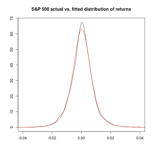
…and now, comparing the theoretical distribution to the actual, things look much closer, particularly at the extremes:

plot(density(sp500.hist.ret),
             xlim=c(-0.04,0.04),xlab="",ylab="",
             main="S&P 500 actual vs. fitted distribution of returns")
x.range <- seq(-0.05,0.05,0.001)
points(x=x.range,y=dnst(x.range, l=nst.pars["l"],s=nst.pars["s"],df=nst.pars["df"]),
       type="l", col="red")

plot(x=density(sp500.hist.ret)$x,y=log(density(sp500.hist.ret)$y),
     xlim=c(-0.04,0.04),ylim=c(-10,5),xlab="",ylab="",type="l",
     main="S&P 500 actual (black) vs. fitted (red) log distribution of returns")
points(x=x.range,
       y=log(dnst(x=x.range,l=nst.pars["l"],s=nst.pars["s"],df=nst.pars["df"])),
       type="l", col="red")

Similarly to how we did things with the normal distribution, we can now determine how likely an event like Black Monday was, given that returns for the market are Student-t distributed, using the desired cutoff value. (-0.22 or -22%)

plot(x=density(sp500.hist.ret)$x,y=log(density(sp500.hist.ret)$y),
     xlim=c(-0.25,0.06),ylim=c(-35,5),xlab="",ylab="",
     main="S&P 500 actual (black) vs. fitted (red) log distribution of returns",type="l")
x.range <- seq(-0.27,0.08,0.001)
points(x=x.range,y=log(dnst(x.range, l=nst.pars["l"],s=nst.pars["s"],df=nst.pars["df"])),
       type="l", col="red")
abline(v=sp500.bm.ret,col="blue")

pnst <- function(q, l, s, df) {return(pt(as.numeric((q-l)/s), df))}
1/pnst(q=sp500.bm.ret,l=nst.pars["l"],s=nst.pars["s"],df=nst.pars["df"])

## [1] 2757592

So, if we assume that S&P 500 returns are Student-t distributed, we would expect an event at least as extreme as Black Monday every 2,757,592 trading days, or once in about 11,000 years. This answer seems a lot more reasonable than the once every 4.03 × 10¹⁸¹ trading days result we got assuming a normal distribution: the Student-t-based model says that Black Monday was very, very unlikely, but not impossible.

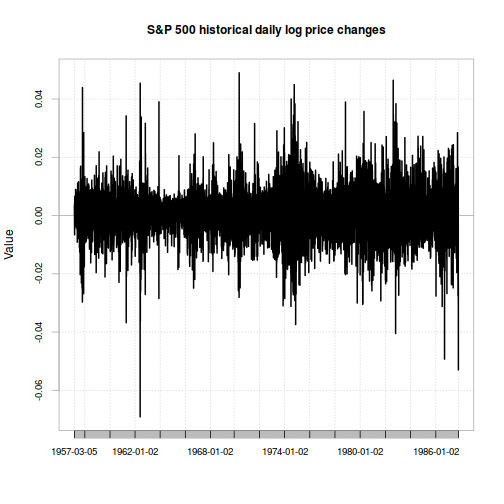
While this estimation method certainly seems to work better than the normal distribution assumption, it still has some issues. For one thing, both the normal and Student-t approaches assume that the market's distribution of risk is constant. But looking at a chart of daily returns, it definitely looks like there are some periods with higher volatility and some with lower:

chart.TimeSeries(xts(sp500.hist.ret,
                     index(sp500.hist)[2:length(index(sp500.hist))]),
                 main="S&P 500 historical daily log price changes")

It turns out you can model this too… click to the next article to see how.

1: You're probabily familiar with seeing actual distributions plotted as histograms. Here, I've plotted the actual distribution of returns as a kernel density estimator instead. One advantage they have is that they're continuous, which can make them easier to compare with theoretical distribtions. See this link for an overview.
2: The normal distribution is not always a bad choice - it depends on what you're doing.
3: Specifically, as the degree-of-freedom parameter approaches infinity, the Student-t distribution approaches the normal distribution.
4: Careful - the scale parameter in the Student-t distribution is similar to, but not the same as the normal distribution's variance parameter!

Black Monday: How unlikely was it, and could it happen again? (Part I)

This post is the first in a series that will look back on the events of Black Monday, which happened 30 years ago today, and explore how it might be relevant to contemporary investing. It makes for a fascinating educational case study that weaves together lessons in finance, statistics, coding, and history. Throughout this series, I'll be “showing my work” with R code that you can run yourself. (For example, in RStudio)

The S&P 500 had seen a new all-time high only six weeks previously, but the week of October 12th, 1987 did not go well for the US stock market. After Monday and Tuesday saw a small loss followed by a small gain, the rest of the week saw mounting losses: 3% on Wednesday, 2% on Thursday, and an alarming and very unusual 5% on Friday.

Still, few were prepared for what happened when the market re-opened on Monday the 19th. The S&P 500 began falling quickly after the open, and continued to do so almost unabated throughout the entire trading day. (See this WSJ interactive for how things unfolded during the day.) When the dust settled at the close, the index had dropped an astonishing 20%. This drop was and continues to be unprecedented; at no other time in its 60-year history has the index dropped even half as much. Monday the 19th, 1987 has since become known as “Black Monday”, one of only a handful of trading dates to receive names and by far the most well known.

As with all disasters, a natural question to ask is, “could it happen again?” As it turns out, there are a number of different ways to try to answer this question, some of which do a good job of highlighting the challenges and complexities of mathematical finance.

To address the question, “how likely would a repeat (or worse) of Black Monday be?”, you need two things:

(1) A model for the probability that the market will rise or fall by a given amount,
(2) Data for the model, and
(3) Knowledge of the ways in which your model may be imprecise or incomplete.

So, let's begin.

The most basic model commonly used for the distribution of price changes is the log-normal distribution. This model assumes that the change of the natural logarithm of price ( log p_t1 - log p_t0 ) is normally distributed.

The formula for the normal distribution is

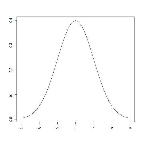
…where τ=2π is the circle constant and μ and σ are the distribution's two parameters, which govern where the peak of the distribution is centered, and how wide it is. For the most basic case of μ=0 and σ=1, the curve looks like this:

x.range <- seq(-3,3,0.01)
plot(x=x.range,y=dnorm(x.range),type="l",xlab="",ylab="")

Now we need to see what real-world data looks like. Conveniently, Yahoo! has a freely-available daily timeseries for the S&P 500.¹

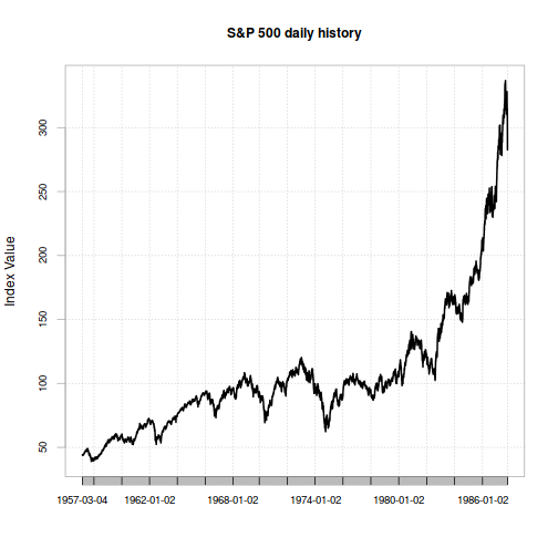
Let's load the data series. Specifically, we'll make one set of data that starts on the official index inception date of March 4, 1957², and ends the day before Black Monday. Then we'll make one more datapoint for Black Monday's return. What does the data look like?

library(quantmod)
library(xts)
library(PerformanceAnalytics)
sp500 <- getSymbols(Symbols="^GSPC",
                    auto.assign=FALSE,
                    from="1957-03-04",
                    to=  "1987-10-20")
sp500.hist <- sp500$GSPC.Close["1957-03-04/1987-10-16",]
chart.TimeSeries(sp500.hist,
                 main="S&P 500 daily history",
                 ylab="Index Value")

For this data, μ=0.000241 and σ=0.00797. For this model, we can determine how likely Black Monday was by plugging in μ, σ, and the desired cutoff value (-0.22 or -22%) into the cumulative distribution function, which will then return the total probability of observing a return that extreme or worse.

sp500.hist.ret.xts <- diff(log(sp500.hist))[is.finite(diff(log(sp500.hist)))]
sp500.hist.ret <- as.numeric(sp500.hist.ret.xts)
sp500.hist.mu <- mean(sp500.hist.ret)
sp500.hist.sd <- sd(sp500.hist.ret)
sp500.bm.ret <- as.numeric(diff(log(sp500$GSPC.Close))["1987-10-19",])
1/pnorm(q=sp500.bm.ret,mean=sp500.hist.mu,sd=sp500.hist.sd)

## [1] 4.03487e+181

So, we'd expect an event as extreme as Black Monday every 4.03 × 10¹⁸¹ trading days.

On the one hand, this explains why the event was such a surprise… the most-commonly-assumed model indicates it was very unlikely! If you're curious about where quotes like “this was an 17 (or 25, etc.) sigma event” come from, take σ and divide it into the % price change to get the number of standard deviations of the move - in this case roughly 29.

On the other hand… while Black Monday may have been unlikely, was it really that unlikely? According to current estimates the universe is only 3.46 × 10¹² trading days old. Was Black Monday really so unlikely that we'd only expect to see it once in 10¹⁶⁹ lifetimes of the universe? Something seems fishy here. Given the frequency with which “Black Swan”, “Unprecedented” events seem to happen in finance, perhaps we can do better than say this was so unlikely as to never happen again, declare victory, and walk away.

To see how we might do better, click over to the next article.

1: Yahoo!'s data series for the S&P 500 doesn't include dividends, but since we're looking at extreme 1-day changes, we can safely ignore their impact in this case – the contribution to returns of dividends is quite small and stable at the daily time scale.
2: For dates before 1962-01-02, the Yahoo! series only has close values; other dates have all of Open, High, Low, and Close. We only use the close prices for these exercises.